Fichier:Mplwp universe scale evolution.svg

Taille de cet aperçu PNG pour ce fichier SVG : 600 × 450 pixels. Autres résolutions : 320 × 240 pixels | 640 × 480 pixels | 1 024 × 768 pixels | 1 280 × 960 pixels | 2 560 × 1 920 pixels.
Fichier d’origine (Fichier SVG, nominalement de 600 × 450 pixels, taille : 57 kio)
Ce fichier et sa description proviennent de Wikimedia Commons.
Description
| Description |
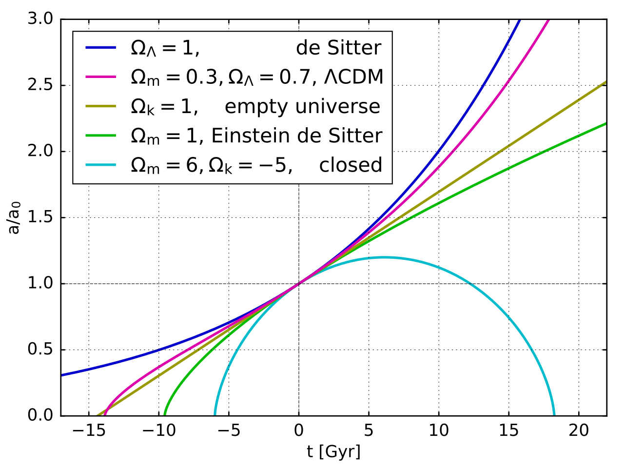
English: Plot of the evolution of the size of the universe (scale parameter a) over time (in billion years, Gyr). Different models are shown, which are all solutions to the Friedmann equations with different parameters. The evolution is governed by the equation
Here is the radiation density, the matter density, the curvature parameter and the dark energy, all normalized such that represents the fact that today's expansion rate is .
|
| Date | |
| Source | Travail personnel |
| Auteur | Geek3 |
| SVG information | |
| Code source | Python code#!/usr/bin/python
# -*- coding: utf8 -*-
import matplotlib.pyplot as plt
import matplotlib as mpl
import numpy as np
from math import *
code_website = 'http://commons.wikimedia.org/wiki/User:Geek3/mplwp'
try:
import mplwp
except ImportError, er:
print 'ImportError:', er
print 'You need to download mplwp.py from', code_website
exit(1)
name = 'mplwp_universe_scale_evolution.svg'
fig = mplwp.fig_standard(mpl)
fig.set_size_inches(600 / 72.0, 450 / 72.0)
mplwp.set_bordersize(fig, 58.5, 16.5, 16.5, 44.5)
xlim = -17, 22; fig.gca().set_xlim(xlim)
ylim = 0, 3; fig.gca().set_ylim(ylim)
mplwp.mark_axeszero(fig.gca(), y0=1)
import scipy.optimize as op
from scipy.integrate import odeint
tH = 978. / 68. # Hubble time in Gyr
def Hubble(a, matter, rad, k, darkE):
# the Friedman equation gives the relative expansion rate
a = a[0]
if a <= 0: return 0.
r = rad / a**4 + matter / a**3 + k / a**2 + darkE
if r < 0: return 0.
return sqrt(r) / tH
def scale(t, matter, rad, k, darkE):
return odeint(lambda a, t: a*Hubble(a, matter, rad, k, darkE), 1., [0, t])
def scaled_closed_matteronly(t, m):
# analytic solution for matter m > 1, rad=0, darkE=0
t0 = acos(2./m-1) * 0.5 * m / (m-1)**1.5 - 1. / (m-1)
try: psi = op.brentq(lambda p: (p - sin(p))*m/2./(m-1)**1.5
- t/tH - t0, 0, 2 * pi)
except Exception: psi=0
a = (1.0 - cos(psi)) * m * 0.5 / (m-1.)
return a
# De Sitter http://en.wikipedia.org/wiki/De_Sitter_universe
matter=0; rad=0; k=0; darkE=1
t = np.linspace(xlim[0], xlim[-1], 5001)
a = [scale(tt, matter, rad, k, darkE)[1,0] for tt in t]
plt.plot(t, a, zorder=-2,
label=ur'$\Omega_\Lambda=1$, de Sitter')
# Standard Lambda-CDM https://en.wikipedia.org/wiki/Lambda-CDM_model
matter=0.3; rad=0.; k=0; darkE=0.7
t0 = op.brentq(lambda t: scale(t, matter, rad, k, darkE)[1,0], -20, 0)
t = np.linspace(t0, xlim[-1], 5001)
a = [scale(tt, matter, rad, k, darkE)[1,0] for tt in t]
plt.plot(t, a, zorder=-1,
label=ur'$\Omega_m=0.\!3,\Omega_\Lambda=0.\!7$, $\Lambda$CDM')
# Empty universe
matter=0; rad=0; k=1; darkE=0
t0 = op.brentq(lambda t: scale(t, matter, rad, k, darkE)[1,0], -20, 0)
t = np.linspace(t0, xlim[-1], 5001)
a = [scale(tt, matter, rad, k, darkE)[1,0] for tt in t]
plt.plot(t, a, label=ur'$\Omega_k=1$, empty universe', zorder=-3)
'''
# Open Friedmann
matter=0.5; rad=0.; k=0.5; darkE=0
t0 = op.brentq(lambda t: scale(t, matter, rad, k, darkE)[1,0], -20, 0)
t = np.linspace(t0, xlim[-1], 5001)
a = [scale(tt, matter, rad, k, darkE)[1,0] for tt in t]
plt.plot(t, a, label=ur'$\Omega_m=0.\!5, \Omega_k=0.5$')
'''
# Einstein de Sitter http://en.wikipedia.org/wiki/Einstein–de_Sitter_universe
matter=1.; rad=0.; k=0; darkE=0
t0 = op.brentq(lambda t: scale(t, matter, rad, k, darkE)[1,0], -20, 0)
t = np.linspace(t0, xlim[-1], 5001)
a = [scale(tt, matter, rad, k, darkE)[1,0] for tt in t]
plt.plot(t, a, label=ur'$\Omega_m=1$, Einstein de Sitter', zorder=-4)
'''
# Radiation dominated
matter=0; rad=1.; k=0; darkE=0
t0 = op.brentq(lambda t: scale(t, matter, rad, k, darkE)[1,0], -20, 0)
t = np.linspace(t0, xlim[-1], 5001)
a = [scale(tt, matter, rad, k, darkE)[1,0] for tt in t]
plt.plot(t, a, label=ur'$\Omega_r=1$')
'''
# Closed Friedmann
matter=6; rad=0.; k=-5; darkE=0
t0 = op.brentq(lambda t: scaled_closed_matteronly(t, matter)-1e-9, -20, 0)
t1 = op.brentq(lambda t: scaled_closed_matteronly(t, matter)-1e-9, 0, 20)
t = np.linspace(t0, t1, 5001)
a = [scaled_closed_matteronly(tt, matter) for tt in t]
plt.plot(t, a, label=ur'$\Omega_m=6, \Omega_k=\u22125$, closed', zorder=-5)
plt.xlabel('t [Gyr]')
plt.ylabel(ur'$a/a_0$')
plt.legend(loc='upper left', borderaxespad=0.6, handletextpad=0.5)
plt.savefig(name)
mplwp.postprocess(name)
|


Conditions d’utilisation
Moi, en tant que détenteur des droits d’auteur sur cette œuvre, je la publie sous la licence suivante :
Ce fichier est sous la licence Creative Commons Attribution – Partage dans les Mêmes Conditions 4.0 International.
- Vous êtes libre :
- de partager – de copier, distribuer et transmettre cette œuvre
- d’adapter – de modifier cette œuvre
- Sous les conditions suivantes :
- paternité – Vous devez donner les informations appropriées concernant l'auteur, fournir un lien vers la licence et indiquer si des modifications ont été faites. Vous pouvez faire cela par tout moyen raisonnable, mais en aucune façon suggérant que l’auteur vous soutient ou approuve l’utilisation que vous en faites.
- partage à l’identique – Si vous modifiez, transformez, ou vous basez sur cette œuvre, vous devez distribuer votre contribution sous la même licence ou une licence compatible avec celle de l’original.
Historique du fichier
Cliquer sur une date et heure pour voir le fichier tel qu'il était à ce moment-là.
| Date et heure | Vignette | Dimensions | Utilisateur | Commentaire | |
|---|---|---|---|---|---|
| actuel | 17 avril 2017 à 02:12 | | 600 × 450 (57 kio) | Geek3 | validator fix |
| 17 avril 2017 à 00:33 |  | 600 × 450 (57 kio) | Geek3 | {{Information |Description ={{en|1=Plot of the evolution of the size of the universe (scale parameter ''a'') over time (in billion years, Gyr). Different models are shown, which are all solutions to the {{W|Friedmann equations|Friedmann equations}}... |
Utilisation du fichier
La page suivante utilise ce fichier :
Usage global du fichier
Les autres wikis suivants utilisent ce fichier :
- Utilisation sur ar.wikipedia.org
- Utilisation sur az.wikipedia.org
- Utilisation sur bg.wikipedia.org
- Utilisation sur de.wikipedia.org
- Utilisation sur en.wikipedia.org
- Utilisation sur es.wikipedia.org
- Utilisation sur fa.wikipedia.org
- Utilisation sur hr.wikipedia.org
- Utilisation sur it.wikipedia.org
- Utilisation sur it.wikiquote.org
- Utilisation sur sr.wikipedia.org
- Utilisation sur ta.wikipedia.org
- Utilisation sur vi.wikipedia.org