Fichier:Kernel trick idea.svg

Taille de cet aperçu PNG pour ce fichier SVG : 800 × 343 pixels. Autres résolutions : 320 × 137 pixels | 640 × 274 pixels | 1 024 × 439 pixels | 1 280 × 549 pixels | 2 560 × 1 097 pixels | 1 344 × 576 pixels.
Fichier d’origine (Fichier SVG, nominalement de 1 344 × 576 pixels, taille : 13 kio)
Ce fichier et sa description proviennent de Wikimedia Commons.
Description
| Description |
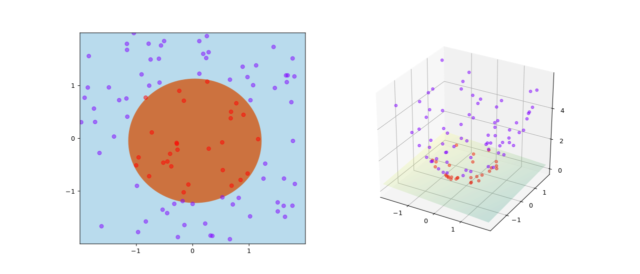
English: An illustration of kernel trick in SVM. Here the kernel is given by:
|
| Date | |
| Source | Travail personnel |
| Auteur | Shiyu Ji |


Python Source Code
import numpy as np
import matplotlib
matplotlib.use('svg')
import matplotlib.pyplot as plt
from sklearn import svm
from matplotlib import cm

# Prepare the training set.
# Suppose there is a circle with center at (0, 0) and radius 1.2.
# All the points within the circle are labeled 1.
# All the points outside the circle are labeled 0.
nSamples = 100
spanLen = 2
X = np.zeros((nSamples, 2))
y = np.zeros((nSamples, ))

for i in range(nSamples):
  a, b = [np.random.uniform(-spanLen, spanLen) for _ in ['x', 'y']]
  X[i][0], X[i][1] = a, b
  y[i] = 1 if a*a + b*b < 1.2*1.2 else 0

# Custom kernel,
def my_kernel(A, B):
  gram = np.zeros((A.shape[0], B.shape[0]))
  for i in range(A.shape[0]):
    for j in range(B.shape[0]):
      assert A.shape[1] == B.shape[1]
      L2A, L2B = 0.0, 0.0
      for k in range(A.shape[1]):
        gram[i, j] += A[i, k] * B[j, k]
        L2A += A[i, k] * A[i, k]
        L2B += B[j, k] * B[j, k]
      gram[i, j] += L2A * L2B
  return gram

# SVM train.
clf = svm.SVC(kernel = my_kernel)
clf.fit(X, y)
coef = clf.dual_coef_[0]
sup = clf.support_
b = clf.intercept_
x_min, x_max = -spanLen, spanLen
y_min, y_max = -spanLen, spanLen
xx, yy = np.meshgrid(np.arange(x_min, x_max, .02), np.arange(y_min, y_max, .02))
Z = clf.predict(np.c_[xx.ravel(), yy.ravel()])
Z = Z.reshape(xx.shape)

# Plot the 2D layout.
fig = plt.figure(figsize = (6, 14))
plt1 = plt.subplot(121)
plt1.set_xlim([-spanLen, spanLen])
plt1.set_ylim([-spanLen, spanLen])
plt1.set_xticks([-1, 0, 1])
plt1.set_yticks([-1, 0, 1])
plt1.pcolormesh(xx, yy, Z, cmap=cm.Paired)
y_unique = np.unique(y)
colors = cm.rainbow(np.linspace(0.0, 1.0, y_unique.size))
for this_y, color in zip(y_unique, colors):
  this_Xx = [X[i][0] for i in range(len(X)) if y[i] == this_y]
  this_Xy = [X[i][1] for i in range(len(X)) if y[i] == this_y]
  plt1.scatter(this_Xx, this_Xy, c=color, alpha=0.5)

# Process the training data into 3D by applying the kernel mapping:
# phi(x, y) = (x, y, x*x + y*y).
X3d = np.ndarray((X.shape[0], 3))
for i in range(X.shape[0]):
    a, b = X[i][0], X[i][1]
    X3d[i, 0], X3d[i, 1], X3d[i, 2] = [a, b, a*a + b*b]

# Plot the 3D layout after applying the kernel mapping.
from mpl_toolkits.mplot3d import Axes3D
plt2 = plt.subplot(122, projection="3d")
plt2.set_xlim([-spanLen, spanLen])
plt2.set_ylim([-spanLen, spanLen])
plt2.set_xticks([-1, 0, 1])
plt2.set_yticks([-1, 0, 1])
plt2.set_zticks([0, 2, 4])
for this_y, color in zip(y_unique, colors):
  this_Xx = [X3d[i, 0] for i in range(len(X3d)) if y[i] == this_y]
  this_Xy = [X3d[i, 1] for i in range(len(X3d)) if y[i] == this_y]
  this_Xz = [X3d[i, 2] for i in range(len(X3d)) if y[i] == this_y]
  plt2.scatter(this_Xx, this_Xy, this_Xz, c=color, alpha=0.5)

# Plot the 3D boundary.
def onBoundary(x, y, z, X3d, coef, sup, b):
  err = 0.0
  n = len(coef)
  for i in range(n):
    err += coef[i] * (x*X3d[sup[i], 0] + y*X3d[sup[i], 1] + z*X3d[sup[i], 2])
  err += b
  if abs(err) < .1:
    return True
  return False

Xr = np.arange(x_min, x_max, .02)
Yr = np.arange(y_min, y_max, .02)
Z = np.zeros(Z.shape)
for i in range(Xr.shape[0]):
  x = Xr[i]
  for j in range(Yr.shape[0]):
    y = Yr[j]
    for z in np.arange(0, 2, .02):
      if onBoundary(x, y, z, X3d, coef, sup, b):
        Z[i, j] = z
        break
plt2.plot_surface(xx, yy, Z, cmap='summer', alpha=0.2)

plt.savefig("kernel_trick_idea.svg", format = "svg")
Conditions d’utilisation
Moi, en tant que détenteur des droits d’auteur sur cette œuvre, je la publie sous la licence suivante :
Ce fichier est sous la licence Creative Commons Attribution – Partage dans les Mêmes Conditions 4.0 International.
- Vous êtes libre :
- de partager – de copier, distribuer et transmettre cette œuvre
- d’adapter – de modifier cette œuvre
- Sous les conditions suivantes :
- paternité – Vous devez donner les informations appropriées concernant l'auteur, fournir un lien vers la licence et indiquer si des modifications ont été faites. Vous pouvez faire cela par tout moyen raisonnable, mais en aucune façon suggérant que l’auteur vous soutient ou approuve l’utilisation que vous en faites.
- partage à l’identique – Si vous modifiez, transformez, ou vous basez sur cette œuvre, vous devez distribuer votre contribution sous la même licence ou une licence compatible avec celle de l’original.
Historique du fichier
Cliquer sur une date et heure pour voir le fichier tel qu'il était à ce moment-là.
| Date et heure | Vignette | Dimensions | Utilisateur | Commentaire | |
|---|---|---|---|---|---|
| actuel | 17 juillet 2020 à 16:41 | | 1 344 × 576 (13 kio) | SemperVinco | Optimized svg code |
| 28 juin 2017 à 08:08 |  | 1 260 × 540 (8,06 Mio) | Shiyu Ji | Reverted to version as of 05:28, 28 June 2017 (UTC) | |
| 28 juin 2017 à 08:05 |  | 540 × 1 260 (7,33 Mio) | Shiyu Ji | vertical for better display | |
| 28 juin 2017 à 07:28 |  | 1 260 × 540 (8,06 Mio) | Shiyu Ji | User created page with UploadWizard |
Utilisation du fichier
Les 2 pages suivantes utilisent ce fichier :
Usage global du fichier
Les autres wikis suivants utilisent ce fichier :
- Utilisation sur ca.wikipedia.org
- Utilisation sur de.wikipedia.org
- Utilisation sur en.wikipedia.org
- Utilisation sur es.wikipedia.org
- Utilisation sur fa.wikipedia.org
- Utilisation sur it.wikipedia.org
- Utilisation sur ja.wikipedia.org
- Utilisation sur ru.wikipedia.org
- Utilisation sur sr.wikipedia.org
- Utilisation sur uk.wikipedia.org
- Utilisation sur zh.wikipedia.org